Scaling Spatial Pipelines: Why Your Location Queries Are Crashing (And How We Fix Them)
A behind-the-curtain look at the infrastructure decisions and optimization secrets we use to build enterprise-grade spatial systems.
When location queries crash production servers, improper bounding-box indexing and unconstrained spatial joins are almost always the culprit. This guide covers how to restructure PostGIS performance, utilize ST_DWithin with spatial indexes, and implement a decoupled storefront architecture. Explore our dedicated PostGIS Performance Optimization, Spatial Data Engineering, and PostGIS Consulting Stack.
At Infryne TechWorks, our core mission is simple: We Turn Raw Data Into Spatial Intelligence. But there is a massive difference between plotting a few thousand coffee shops on a map and running real-time proximity analytics on hundreds of millions of geographic records.
As location-based applications scale, standard database architectures inevitably begin to crack under the weight of multi-dimensional queries. The results are universal: sluggish API load times, skyrocketing compute costs, and crashing data pipelines.
When we take on a project struggling with severe spatial bottlenecks, we don't just throw more RAM at the problem — we completely rethink the architecture. Here is a look behind the curtain at the infrastructure decisions and optimization secrets we use to build enterprise-grade spatial pipelines.
The Great Infrastructure Debate: AWS RDS vs. Self-Hosted EC2
When evaluating a struggling database, the first thing we look at is where the data lives. A managed service such as AWS RDS can reduce operational work. AWS documents support for Multi-AZ deployments, read replicas, snapshots, backups, and point-in-time restores in its RDS for PostgreSQL guide.
RDS still has service boundaries and less host-level control than self-managed PostgreSQL. Its current storage documentation lists up to 64 TiB for most PostgreSQL DB instance classes, with lower limits for some instance families, so architecture decisions should use the limits for the selected class and storage type.
Self-hosting grants complete control over PostgreSQL configuration tuning and lets you utilize niche extensions that RDS may not support. More importantly, it supercharges your data ingestion — running ingestion processes locally on the database server makes commands like \copy significantly faster than piping massive datasets over the network into RDS.
The trade-off: self-hosting requires high DevOps maturity. Your team becomes entirely responsible for replication, failovers, and disaster recovery.
Rethinking PostGIS: The "Storefront" Pattern
Once the infrastructure is decided, we bring in PostGIS — the gold standard for spatial databases. However, the biggest mistake we see development teams make is using PostGIS for everything.
PostGIS is incredibly powerful, but it should not be used as your massive-scale, raw data-crunching factory. Using it this way leads to degraded performance, high memory pressure, and unpredictable query times at scale.
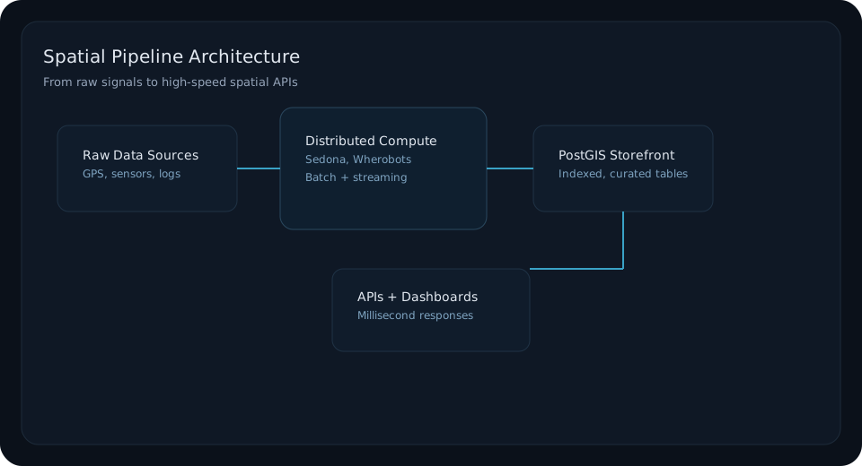
Instead, we implement a modern spatial pipeline pattern. Distributed engines can handle batch-oriented transformations before serving curated results from PostGIS. The Apache Sedona documentation describes spatial DataFrame, SQL, raster, vector, indexing, and distributed-query capabilities across Spark and Flink.
In this architecture, PostGIS acts strictly as your "high-speed storefront." Once the distributed tools process the raw data, we load those refined spatial insights into PostGIS. Its only job is to serve those insights to your end-users via your APIs with lightning speed.
Indexing and the ST_DWithin Secret
Even with perfect infrastructure, bad queries will bring your application to a halt. When a client tells us their spatial queries take minutes to load, we immediately look at two things: their indexes and their math.
Incredible for massive tables. Takes up virtually no storage (kilobytes, not megabytes) and builds blazing fast — but only effective if your data is stored in a highly spatially correlated order.
The general-purpose multi-dimensional spatial index. If your data is scattered or you can't guarantee sequential spatial ordering, GiST is the reliable choice.
The most common anti-pattern we fix is the proximity search. Previous developers often use ST_Buffer+ST_Intersects, or put ST_Distance directly in a WHERE clause — forcing the database to perform complex geometric math on every single row in the table. This is a catastrophic performance killer.
For radius filtering, use ST_DWithin when its semantics fit the query. PostGIS documents that it includes a bounding-box comparison that can use available spatial indexes before the exact distance test. Measure the resulting plan with EXPLAIN (ANALYZE, BUFFERS); improvement depends on data distribution, selectivity, and configuration.
Kernel & PostgreSQL Memory Parameters for Spatial Workloads
Out-of-the-box PostgreSQL configurations are famously conservative, tuned to run on 1990s hardware with 128 MB of RAM. When hosting multi-gigabyte spatial datasets with complex polygon geometries, default settings trigger constant disk spilling and catastrophic cache thrashing.
Here is the baseline postgresql.conf configuration we deploy on production 64 GB RAM spatial database servers (such as AWS EC2 r6i.2xlarge):
# Memory Configuration (64 GB RAM Host)
shared_buffers = 16GB                  # 25% of total system memory for PG buffer cache
effective_cache_size = 48GB            # 75% of RAM, informs planner of OS file cache
work_mem = 64MB                        # Dedicated sort & hash memory per query operation
maintenance_work_mem = 2GB             # Accelerates CREATE INDEX (GiST / SP-GiST builds)

# Storage & Planner Tuning for NVMe SSDs
random_page_cost = 1.1                 # Matches sequential scan cost on modern NVMe drives
effective_io_concurrency = 200         # Allows asynchronous pre-fetching on SSD arrays
seq_page_cost = 1.0

# Parallel Query Execution
max_worker_processes = 8
max_parallel_workers = 8
max_parallel_workers_per_gather = 4    # Enables parallel spatial index scans and joins
parallel_tuple_cost = 0.05PostgreSQL default random_page_cost = 4.0 assumes spinning rotational hard disks where random seeks were 4x more expensive than sequential reads. On modern cloud NVMe storage (such as AWS gp3 or io2), random read penalty is virtually zero. Leaving it at 4.0 causes the query planner to mistakenly assume a sequential table scan is cheaper than a GiST index lookup, completely bypassing your spatial indexes!
The Geometry vs. Geography Trap: Projections & Distortion
One of the most insidious bugs in geospatial software is confusing planar geometry with ellipsoidal geography. PostGIS provides two foundational spatial types:
Operates on a flat Cartesian plane (x, y). All distance and area functions assume flat Euclidean geometry: d = √(Δx² + Δy²).
Operates on the curved surface of the WGS 84 ellipsoid (EPSG:4326). Calculates true geodesic distances along the Earth's curve.
If your table is stored in geometry(Point, 4326) and a developer writes ST_Buffer(geom, 1000) expecting a 1,000-meter buffer, they have actually requested a buffer of 1,000 angular degrees — wrapping around the Earth nearly three times and crashing the database thread!
Even writing ST_Buffer(geom, 0.01) (assuming 1 km) causes severe distortion: 0.01 degrees is ~1,113 meters at the Equator, but shrinks to only ~715 meters at 50° latitude (London/Frankfurt) due to meridian convergence.
-- WRONG: Planar distance on unprojected degrees (Slow, inaccurate, non-indexed)
SELECT id, name
FROM stores
WHERE ST_Distance(geom, ST_SetSRID(ST_MakePoint(-73.985, 40.748), 4326)) < 0.01;

-- RIGHT: Native geodesic proximity with spatial index acceleration
SELECT id, name
FROM stores
WHERE ST_DWithin(geom::geography, ST_MakePoint(-73.985, 40.748)::geography, 1000);

-- ALTERNATIVE: Project to localized UTM zone for lightning-fast Cartesian math
SELECT id, name
FROM stores
WHERE ST_DWithin(
  ST_Transform(geom, 32618),  -- UTM Zone 18N (New York, meters)
  ST_Transform(ST_SetSRID(ST_MakePoint(-73.985, 40.748), 4326), 32618),
  1000
);
Benchmarking the ST_DWithin Secret: Real Execution Plans
To demonstrate the astronomical performance gap, we benchmarked a dataset of 10,000,000 geospatial vehicle location pings on an AWS r6i.xlarge instance.
EXPLAIN (ANALYZE, BUFFERS)
SELECT id FROM telemetry
WHERE ST_Distance(geom, ST_MakePoint(55.27, 25.20)) < 0.05;EXPLAIN (ANALYZE, BUFFERS)
SELECT id FROM telemetry
WHERE ST_DWithin(geom::geography, ST_MakePoint(55.27, 25.20)::geography, 5000);Why is ST_DWithin 1,500 times faster? Because ST_DWithin automatically injects a bounding box envelope operator (&&) into the query tree before executing distance calculations. The R-Tree / GiST index instantly discards 99.9% of candidate rows using fast integer bounding-box math, evaluating expensive spherical trigonometry on only the few dozen coordinates that actually fall inside the bounding square!
ST_Subdivide: Taming Giant Complex Polygons
Here is a common failure mode in spatial joins: You have a table of 50 million delivery addresses and want to spatial-join them against municipal boundaries or national forest parcels. Each polygon contains 20,000 to 100,000 vertices (e.g., highly detailed coastlines or jagged riverbanks). The spatial query takes 45 minutes and runs out of memory.
The problem is Bounding Box Bloat. A giant polygon spanning an entire province has a massive bounding box covering thousands of irrelevant points. Every single point inside that enormous box must undergo vertex-by-vertex point-in-polygon ray-casting tests.
-- Step 1: Subdivide complex polygons into compact tiles (max 256 vertices each)
CREATE TABLE municipal_boundaries_subdivided AS
SELECT
  id AS original_id,
  name,
  province_code,
  ST_Subdivide(geom, 256) AS geom
FROM municipal_boundaries;

-- Step 2: Build a GiST index on the subdivided geometry
CREATE INDEX idx_mun_subdivided_geom
ON municipal_boundaries_subdivided USING GIST(geom);

-- Step 3: Run the spatial join (Executes in seconds instead of minutes!)
SELECT
  p.id AS ping_id,
  m.name AS municipality
FROM vehicle_pings p
JOIN municipal_boundaries_subdivided m
  ON ST_Intersects(p.geom, m.geom);
By subdividing complex polygons into smaller bounding boxes with at most 256 vertices, the GiST index can precisely isolate which micro-polygon actually intersects each point. The point-in-polygon test executes in microseconds instead of milliseconds, cutting overall join duration by up to 95%.
Spatial Indexing Decision Tree: GiST vs. SP-GiST vs. BRIN
Not all spatial indexes are created equal. Choosing the wrong index type can inflate your database size by tens of gigabytes or cripple write throughput during streaming ingestion.
| Index Type | Internal Structure | Storage Overhead | Best Used For | Failure Mode |
|---|---|---|---|---|
| GiST (R-Tree) | Hierarchical bounding boxes | High (~20–35% of table) | Default general-purpose index for points, lines, polygons | High lock contention on ultra-fast concurrent INSERTs |
| SP-GiST (Quad-Tree) | Space-partitioned non-overlapping cells | Medium (~15–20% of table) | Dense point clouds, LiDAR, clustered GPS points | Does not support polygon overlap geometries |
| BRIN (Block Ranges) | Min/Max coordinates per 128 disk blocks | Ultra Low (<1% of table) | Tables 100M+ rows naturally sorted by geography or timestamp | Completely ineffective if data is inserted in random spatial order |
PostGIS vs. MongoDB for Geospatial Workloads: When Documents Fail
A frequent debate among backend engineering teams is choosing PostGIS vs MongoDB spatial. MongoDB provides geospatial queries via GeoJSON and 2dsphere indexes, which works well for basic mobile app features like finding the nearest driver or coffee shop within a bounding radius. But when workloads demand spatial joins, polygon overlays, raster analysis, or national projection transformations, MongoDB hits hard limitations.
| Feature / Capability | PostgreSQL / PostGIS | MongoDB (2dsphere) |
|---|---|---|
| Spatial Index Types | GiST, SP-GiST, BRIN, R-Tree | 2dsphere (S2 grid) & 2d flat |
| CRS / Projection Support | 5,000+ EPSG projections with ST_Transform | WGS 84 (EPSG:4326) only |
| Relational Spatial Joins | Native ST_Intersects, ST_Contains across tables | Limited $lookup with $geoNear restrictions |
| Topological Operations | ST_Buffer, ST_Union, ST_Voronoi, ST_Subdivide | Not supported (requires app-layer logic) |
| Vector Tile Generation | Native binary MVT via ST_AsMVT() | Requires external tiling middleware |
| Licensing & Cost | 100% Free Open Source (GPLv2 / PostgreSQL) | SSPL (Commercial licenses for cloud / Atlas) |
If your application only needs simple point-radius lookups in a single document collection, MongoDB is convenient. However, if your system involves GIS geometry validation, spatial joins, multi-layer analytics, or complex projections, PostGIS remains the gold standard.
Frequently Asked Questions
- Is PostGIS free to use in production?
- Yes. PostGIS is completely free, open-source software licensed under the GNU General Public License (GPLv2). It can be used in commercial and enterprise applications with zero licensing or subscription fees.
- Is PostGIS better than MongoDB for geospatial data?
- For serious spatial analytics, topological relationships, polygon intersections, and CRS re-projections, PostGIS is vastly superior. While MongoDB provides basic 2dsphere proximity lookups on WGS 84 points, PostGIS supports over 5,000 spatial coordinate systems, complex spatial joins, raster processing, and full OGC compliance.
- Why are spatial queries in PostGIS slow?
- Spatial queries typically slow down due to missing GiST or BRIN indexes, using non-indexable functions like ST_Distance in WHERE clauses instead of index-accelerated ST_DWithin, spatial data fragmentation, or using PostGIS as an un-optimized raw ETL compute engine rather than a query storefront.
Ready to Scale?
Optimize Your Spatial Infrastructure
Whether you're deciding between AWS RDS and EC2, struggling with lagging API endpoints, or need to build a distributed spatial pipeline from scratch — your architecture matters.
Primary Sources & Datasets
Continue Reading
More engineering research from Infryne TechWorks
Wildfire burn scar mapping using Sentinel-2 and Landsat 8/9 — NBR, BAIS2, RBR spectral indices, NASA FIRMS active fire integration, and the Infryne TechWorks satellite analytics platform.
A 10-year Landsat archive study overlaying land surface temperature with census wards, income proxies, and tree canopy to map spatial heat burden in Karachi.
A production walkthrough of Sentinel-2 L2A, cloud masking, median composites, spatial validation, CNN inference, and field-ready crop stress alerts.
A practical guide to detecting spatial leakage, choosing geography-aware validation strategies, and building machine-learning evaluations that survive deployment.
A practical guide to WebGL rendering, PMTiles, custom GLSL layers, feature state, performance tuning, Martin, and production-ready Next.js setup.
A production field guide to AWS Batch array jobs, container memory failures, IAM roles, S3 request smoothing, and scaling imagery processing to 10,000 tiles.
A deep technical guide on cloud-native GIS stacks, PMTiles on Cloudflare R2, Rust-powered Martin services, and PostGIS performance tuning.